
Every conversation about Aerochrome eventually arrives at the same sigh: the film is gone, the last boxes were expired, and whatever magenta canopy you remember is now a scarcity story. I want to argue the opposite case from first principles. The look was a set of output relationships between infrared, visible color, and neutral tone. Relationships can be written down. And once they are written down as a lookup table, they behave far more predictably than any surviving roll ever did.
The Palette Was a Relationship, Never a Roll
Strip away the mythology and the Aerochrome signature reduces to three statements. Infrared-rich canopy stays red-magenta. Low-infrared sky stays cyan. Neutral subjects never acquire the same intensity as foliage. That is the whole contract.
A lookup table honors that contract in a way expired emulsion cannot. Identical normalized RGB inputs receive identical mappings, frame after frame, body after body. Aged film gave you batch variance, storage variance, and processing variance stacked on top of each other, and you discovered the result weeks later.
So judge your work accordingly. Compare repeated frames of the same sunlit foliage, the same open sky, and the same neutral target rather than holding your screen up against a scan from an unrelated film batch. Compare LUT versions under one RAW profile, one white-balance method, and one working color space. Otherwise you will read input-pipeline drift as palette drift and start correcting a problem you do not have.
Most digital recreations stall here. They chase a memory of a print instead of locking a mapping.
Where the Red-Blue Swap Runs Out of Road
The channel swap is the first thing everyone tries. I tried it too, and rejected it quickly, because swapping red and blue only relocates channels that the sensor already recorded. It cannot recreate the asymmetric routing the film performed between near-infrared, visible red, and visible green.
The tell is in the leaves. A swap gives you flat inverted red. Aerochrome-style mapping routes infrared-rich foliage toward the red output while visible green still contributes to the blue output, which is exactly why leaves land in pink and magenta rather than a uniform scarlet.
One-click infrared presets fail in a different direction. They crush bark, pavement, and midtone architecture into neon sludge, and because they were built against one camera's infrared response, they do not travel.
The more useful diagnostic is to inspect foliage, bark, pavement, and sky separately, then build a three-anchor map you can save, version, and revise instead of repairing each frame by eye.
Three Anchors, Not OneSunlit foliage sets magenta placement. Clear sky sets cyan placement. A gray card or skin reference enforces restraint through the midtones. If your grade only satisfies two of the three, it will collapse the first time you photograph a person under a tree.
Layer Logic: Why Healthy Leaves Belong in Magenta
The theoretical brief for the LUT comes straight from how the film's layers handed information to each other. Near-infrared exposure supplied the red-rendering component. Visible red contributed toward green. Visible green contributed toward blue.
Now consider a healthy leaf. It reflects near-infrared strongly and it reflects visible green, so its output carries both a red component and a blue component. Magenta is the arithmetic consequence, not a stylistic choice.
Clear sky and open water contribute comparatively little infrared and stay dominated by shorter visible wavelengths, which is why they settle toward cyan and hold there.
Treat foliage as a two-component anchor: strong red output from near-infrared, plus enough blue output from visible green to prevent a featureless scarlet mass. The neutral reference exists so the transform stops pushing every middle-luminance surface into the same saturated false color.
Building the .CUBE Around a Controlled Test Scene
The master file starts as a white-balanced RAW of a scene you constructed on purpose: sunlit leaves, unobstructed blue sky, and a gray card sitting in the same light. Capture it with a full-spectrum body or through a 590-nanometer long-pass filter, and record both the filter and the camera body in the eventual LUT name.
Set exposure so reflective foliage does not clip, then open the file in a fixed RGB working space and stay there.
- Use Curves to establish channel placement for each anchor.
- Use Channel Mixer for the broader infrared-to-red and green-to-blue routing.
- Apply restrained selective adjustments only to separate the three anchors from one another.
- Export the stack as a .CUBE through Photoshop's Color Lookup workflow.
Keep local contrast, sharpening, grain, glow, and vignetting outside the table. Encode global hue placement and relative saturation, nothing else, so the LUT can travel between frames without dragging a mood along with it.
Then verify. Apply the exported .CUBE to a fresh copy of the test file and toggle the Color Lookup layer rather than assuming the export matches the construction stack. Exports lie more often than you would like.
Pipeline Comes FirstThe table is repeatable only inside a normalized capture pipeline. Change the camera's infrared response, the filter transmission, the RAW profile, or the working color space, and the three anchors move before your LUT ever touches them.
Two Baselines: 590-Nanometer Files and Full-Spectrum Files
Here is the fault line that catches people. A 590-nanometer capture arrives with deep blue already suppressed and with a stronger visible-red and near-infrared mixture, which puts it close to the film's working mix from the outset. A full-spectrum file still holds broad blue contamination it has no use for.
That leftover blue means one unqualified .CUBE cannot be a trustworthy master for both. Correct the full-spectrum baseline with a pre-curve, or assign it a separate table entirely, before you judge foliage color at all.
Run the matched-pair test. Photograph the same viewpoint in the same light without changing framing, focus, exposure mode, or illumination; moving clouds and wind-blown leaves will make the comparison worthless. Then inspect three outcomes together: magenta separation among leaf species, cyan continuity across the sky, and retained tonal detail in bark or concrete.
Name the tables by input state, such as FS-base and 590-base. Thumbnails of false-color previews look nearly identical, and that is how the wrong table ends up on the wrong file.
Name the Master, Then Shoot to It
My recommendation is unambiguous: finish one master Aerochrome LUT from a controlled foliage-and-sky test, name it something like Aerochrome_590_BodyA_RGBspace_v03.cube, and expose and white-balance every subsequent frame to that table.
Test it on an evenly lit frame, a backlit foliage frame, and a frame containing bark or concrete before you rely on it in the field. Revise the master only when the same color failure shows up across all three conditions, and keep the editable layered test document beside the exported .CUBE so revision is a deliberate act rather than a rebuild from memory.
Stop reinventing the palette on every file. Let the weather, the species, the angle to the sun, and your filter choice supply the variation. The mapping should be the one thing in the frame that does not move.



Reader Comments
The conversation starts with you.
Your Comment