Crafting Vibrant Crimson Foliage Using 590nm Infrared Captures and Custom Camera Profiles

First Light on a 590nm Conversion in the Maple Stand

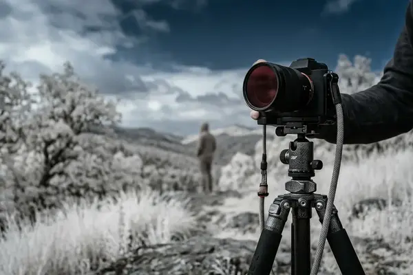
I set the tripod at the maple stand’s edge about 20 minutes before sunrise. The sky had enough brightness to separate the upper branches, while direct light had yet to cross the leaves. Live view on the 590nm-converted body showed a brown-olive canopy with ordinary green largely drained away.

That preview confirmed the spectral capture. It did not promise the finished color.

The conversion filter admits deep visible red and near-infrared. When I release the shutter, the raw file preserves how those wavelengths separate across the sensor’s filtered channels. It still opens in olive-brown, pink-gray, and muted magenta until deliberate channel mapping gives the vegetation a crimson reading.

The Olive-Pink Split

Capture creates the spectral file. The profile, locked white balance, canopy mask, and red-channel curve create the Aerochrome-like interpretation.

This distinction controls the entire workflow. A 590nm conversion supplies useful spectral separation, while crimson foliage remains a post-processing construction.

What a Straight 590nm File Still Withholds from Aerochrome

Why does a converted camera fail to deliver crimson leaves immediately? The 590nm designation describes the conversion filter’s approximate cutoff region. It gives no instruction to map vegetation to red.

The Bayer array continues to produce three channel values, but infrared reaches those filtered channels unevenly. Their responses no longer correspond cleanly to the visible-light meanings of red, green, and blue. A neutral default camera profile interprets the values through assumptions designed for conventional color capture, so foliage commonly settles between muddy olive, dusty rose, and gray-magenta. Auto white balance can shift that uncertain result again.

Define the Intended Separation

Before moving a hue slider, identify the target relationships: a saturated red-magenta canopy, a cooler sky, and trunks or soil that retain their own tonal identity. This turns an attractive color idea into a mapping problem with visible boundaries.

The Kodak Aerochrome palette therefore develops after capture. The raw file contains channel separation that can support the look; it has not yet assigned film-style color meaning to the scene.

A Custom DNG Profile that Reweights 590nm Vegetation

The profile belongs at the start of the color pipeline. If the default profile leaves vegetation scattered across olive and pink, later HSL corrections must pull a broad, unstable range toward crimson. A conversion-specific DNG profile moves that cluster closer to its intended region before local editing begins.

Build the Profile from the Same Optical Path

1. Photograph a 24-patch target with the same 590nm-converted body and lens used for the landscape.
2. Fill enough of the frame for clean patch sampling, and protect the target from clipped highlights or reflected foliage color.
3. Begin with chart-based calibration, then add the creative hue-table or lookup-table adjustment that moves the vegetation cluster toward magenta-red.
4. Name the profile with the converted body and conversion type so it cannot be confused with a visible-light or deeper-infrared profile.
5. Select the profile before setting the final white balance.

The chart establishes reference behavior; the creative table handles the interpretive shift. Keep those functions conceptually separate even when the software stores them in one profile asset.

Match the Conversion

A profile built for this 590nm body-and-lens path should stay with that path. A 720nm or 850nm conversion needs its own profile because its spectral input differs. Even a well-matched digital result remains an Aerochrome-like interpretation rather than a chemical reproduction under every lighting ratio.

Hue-Saturation Layers and the Red Channel After the Profile

Once the custom profile is active, settle the white balance and stop changing it. Temperature or tint adjustments move the foliage range underneath the masks, weakening corrections that appeared precise a moment earlier.

Map the Whole Canopy

Sample at least three foliage areas: a highlight, a midtone, and a shaded leaf group. A mask built from one sunlit patch may omit cooler leaves beneath it or capture unrelated warm surfaces elsewhere. The combined samples should describe the residual olive-to-pink cluster across the canopy’s illumination range.

Apply the correction in a controlled order:

1. Rotate the sampled foliage hue toward crimson.
2. Increase saturation only inside the canopy mask.
3. Inspect bark, soil, sky, and any painted objects before shaping the red channel.
4. Use a shallow red-channel curve or restrained channel-mixer adjustment to refine the final color.

The last step requires restraint. Red-channel shaping should preserve leaf volume, especially where backlighting separates veins from translucent tissue. A large global lift may produce a dramatic thumbnail while stripping structure from the full-resolution file.

Lock Before Layering

Use the fixed sequence: custom DNG profile, white-balance lock, selective foliage correction, then red-channel shaping. Reordering these operations makes masks harder to evaluate and reproduce.

Where an Aggressive Red Push Fractures Leaf Texture

The clearest warning appears at 100% view. Backlit leaves begin to merge into flat red plates, internal veins disappear, and neighboring tones lose separation. The composite histogram may still look acceptable because other channels conceal a red channel pressed against its right boundary.

Audit the Mask and Channel Separately

Temporarily display the foliage mask in monochrome. Bark seams, exposed soil, painted markers, and skin-adjacent warm colors should not carry the same opaque coverage as maple leaves. Review the mask at 100%, then inspect edge transitions at 200% where fine branches cross the canopy.

Next, compare the composite histogram with the individual red channel. If the red channel reaches the right boundary while venation vanishes, reduce the red-channel curve first. Lower saturation second if the foliage still feels compressed. This order protects luminance separation before sacrificing color intensity.

Stop Bark Hitchhiking

When trunks and soil turn red with the maple leaves, the edit has crossed from foliage remapping into indiscriminate channel staining. Tighten the mask rather than trying to neutralize each contaminated object afterward.

A convincing crimson canopy depends on retained texture as much as hue. The file should still describe leaf edges, overlapping planes, and light passing through thin tissue.

Which 590nm Canopy Gets the Crimson Profile First?

Choose one existing 590nm raw landscape with visible separation between foliage and trunks and enough leaf texture to judge the red channel. Make one virtual copy so the straight rendering remains available beside the edited version.

Assign the conversion-specific profile, lock white balance, and test a single masked crimson pass. Judge three regions before expanding the edit: canopy, bark or soil, and sky. The comparison should reveal whether the scene’s tonal structure can support saturated foliage without sacrificing subject separation.

Which 590nm frame in your archive has the leaf texture and clean canopy boundaries to earn that first crimson profile?